What Types of Generative Models Are There?

28 Sep 2020 • 26 mins

Tags: generation 

---

David Donahue  
David is a graduate student at the University of Massachusetts (Lowell), working with Anna Rumshisky. His research focuses on natural language generation.

Introduction

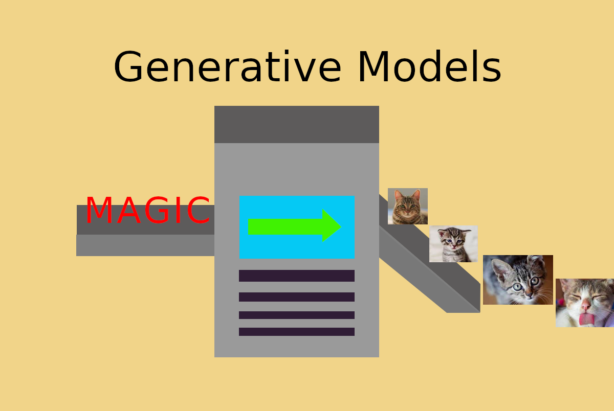
Recently, the field of machine learning has seen a surge in generative modeling - the ability to learn from data to generate complex outputs such as images or natural language. The best models have synthesized photo-realistic images of people who have never existed, Google Translate outputs impressive generative translations between hundreds of languages, and new waveform models are responding to your voice commands with voices of their own. Style transfer models answer the question of how Van Gogh would have painted the Golden Gate bridge. Generative models promise to enrich our world by modeling the complexities of data and bringing forth new patterns we could have never imagined.

So what kinds of generative models are we using nowadays? And why? In this post, we explore these questions and many more answers.

Models we explore in this post

• Discrete modeling
• Recurrent Neural Networks
• Generative Adversarial Networks
• Normalizing Flows
• Variational Autoencoders
• Denoising Score Matching

What do we mean by generative modeling?

If we wish to classify whether that picture on your phone is a cat or a dog, we ask the question: which outcome is the most probable? The straightforward way to go about this is to estimate the probability of both outcomes (this is a cat, this is a dog) using a standard trained neural network and select the option with the highest probability. This is what we refer to as classification, or a discriminative model. We only care about the most probable outcome.

In contrast, generative modeling wishes to sample different outcomes from the distribution. This is not so useful for dogs and cats, as generating random cat and dog labels according to their distribution is not useful or interesting when you look at your photo. There are clear right and wrong answers. But if we want to generate beautiful paintings, we don’t care about the “most probable” painting. We want a beautiful painting similar to what artists actually paint. This is the task: for a dataset of individual paintings x, we want to infer the distribution of all paintings p(x) and then generate new paintings from that distribution.

Types of generative models and their benefits costs

There are a number of properties we want from generative models, such as:

• Stability - how easily can this model be trained?
• Capacity - can this model generate complex data?
• Density - can this model tell us the likelihood of different samples?
• Non-constrained - is the model constrained to a specific structure?
• Speed - is this model slower during training or inference?

Modeling Discrete Distributions

Many classification models attempt to predict some discrete output $Y$. For example, a sentiment analysis system may be fed a fresh tweet and be tasked with predicting its emotion: positive, negative or neutral. This is typically done by learning to represent $P(Y)$, or the probability of different emotions $Y$ for a given input tweet. The selected sentiment is then

$$y* = \underset{y}{\operatorname{argmax}} P(Y=y)$$

But learning $P(Y)$ can also be seen as a generative task, since we could generate different y’s for a given input tweet according to their probability. So how do we learn a generative model $Q(Y)=P(Y)$ given samples from P (our dataset)? Throughout this post, $P$ represents the true distribution of data while $Q$ represents to model estimate of the distribution which we can sample from. We first represent $Q(Y)$ by a neural network $Q(Y) = f(Y)$ for some function $f$. Ideally, we would like to minimize some objective function which, at convergence, brings together the two distributions $Q$ and $P$. For this we use the KL-divergence measure. KL-divergence is defined as follows for distributions $Q$ and $P$.

$$D_{KL}(P\| Q)=\sum_{x} P(x) \log\dfrac{P(x)}{Q(x)}$$

Most notably, as we minimize this KL-divergence measure toward zero, our model $Q$ converges to the true distribution $P$. This is great news, we would have a generative model $Q(x)=P(x)$ (at least theoretically) that could be sampled from. We formulate our objective as follows:

$$\begin{align*} &L = D_{KL}(P \| Q) \\\\ &L = \sum_{x} P(x) \log\dfrac{P(x)}{Q(x)} \\\\ &L = \sum_{x} P(x) (\log P(x)-\log Q(x)) \\\\ &L = \sum_{x} P(x) \log P(x)- \sum_{x} P(x) \log Q(x) \end{align*}$$

This loss function is minimized with respect to $Q$. Since the first term does not depend on Q, it is constant and can be removed:

$$L = -\sum_{x} P(x) \log Q(x) = -E_{x \sim P(x)}[\log Q(x)]$$

And this is the standard cross entropy loss function! We can approximate this with batches of data for learning a distribution in both generation and classification settings. Since this is discrete data we are generating, we can select values according to our probabilities under $Q(x)$. This same objective function will be later used in the “normalizing flow” architecture in a similar way.

Language Modeling

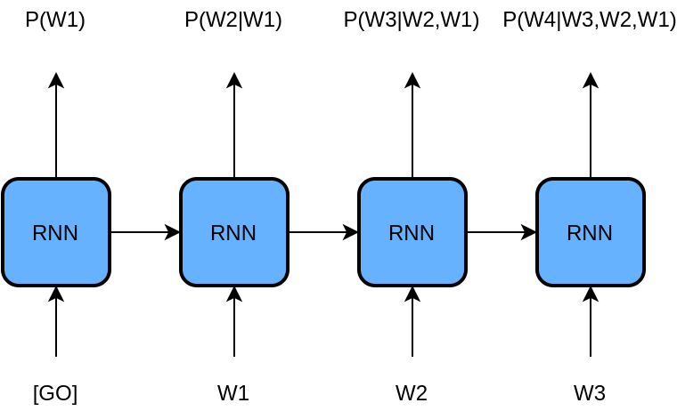
One classic example of generating discrete distributions is the task of language modeling. Specifically, the goal is to generate a natural language sequence of words which is realistic; it sounds like something a human would write. We can model this as a probability distribution over all sequences $P(S)$ according to how likely it is a human would write that sequence (we can add conditioning on input later). The problem is, there is an almost uncountable number of sequences (exponential in sequence length). It is imperative that we find a way to break down the problem. To do this, we take advantage of the fact that a sequence can be broken down into individual words:

$$P(S) = P(w_1, w_2, w_3, w_4) \\$$

Notice that this is a joint distribution over multiple variables, we can factorize the distribution into a series of conditional probabilities to simplify the task:

$$P(S) = P(w_1)P(w_2|w_1)P(w_3|w_2,w_1)P(w_4|w_3,w_2,w_1)$$

Thus, the task now becomes to predict each next word given the previous words. We can model all of these conditional probabilities with a single parameterized model $Q(w_i\vert w_1...w_{i-1})$, called a recurrent neural network (RNN). This RNN predicts each next word given the previous words, and is ubiquitous in the field of natural language processing (NLP) for applications such as document summarization, chatbots, and machine translation (e.g. Google Translate!). Since this setup is still a problem of discrete modeling, we again deploy the cross entropy loss function for training each next-word prediction. For more information on the structure of RNNs, I refer the reader to this wonderful blog post about Long Short-Term Memory networks here and this more recent post on the novel Transformer architecture here.

Fig. 1. Recurrent neural network processing a sequence.

Normalizing Flows

Discrete modeling of probability distributions is vital to the generation of discrete categories and sequences, but how does this scheme apply to real values? Using the discrete setup above, we would require an infinite number of categories, as each real number in the data can take on an infinite number of values. That’s a lot of training data! A great example of this is images, where all pixels in an image have RGB pixels which take on values from 0 to 1 (depending on precision). We can then imagine a high-dimensional “space” of images we can move around in.

Instead of modeling the probability of any discrete value $P(x)$, what if we could instead represent the continuous probability distribution of a real value $p(x)$? (lowercase letters for continuous distributions). Then, we could minimize the same KL-divergence measure above between our $q(x)$ and $p(x)$ to recover $q(x)=p(x)$. Once we learn the distribution, we should also be able to sample from it to produce new data!

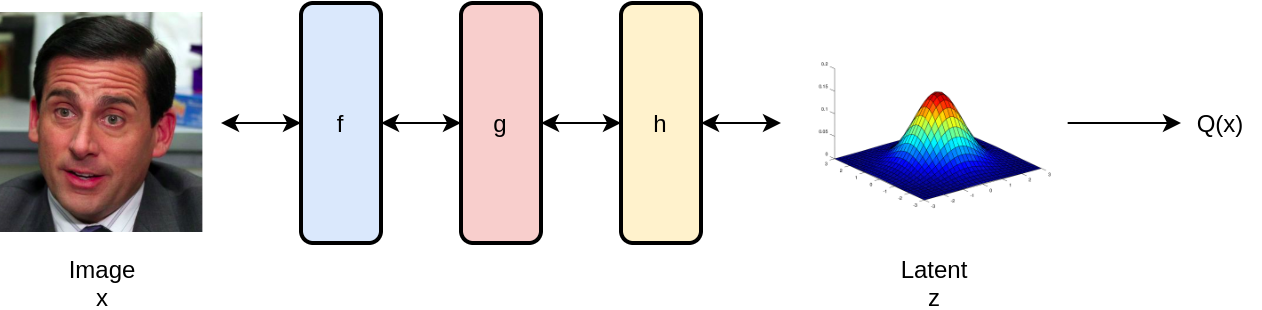
The problem: how do we represent the probability distribution $q(x)$ for an infinite number of values? Here we introduce the normalizing flow (Dinh, Sohl-Dickstein, & Bengio, 2016), which satisfies this question by producing $q(x)$ through a series of transformations on a known continuous distribution. Put simply, we bend a distribution we know into the distribution we desire! We start from say a (multivariate) gaussian distribution, and manipulate it step by step through multiple invertible neural network layers into the distribution of celebrities faces or whatever else we wish to generate. The magic of flows stems from the change of variables formula, which can be used to express one probability distribution in terms of another through a transformation:

$$p(x)=p(z) \bigg\rvert \det (\dfrac{\partial g(z)}{\partial z}) \bigg\rvert^{-1}$$

for an invertible transformation $x = g(z)$. This can be interpreted as saying that the probability density of the output of some function $g(z)$ is determined by the input density and the “scale” of the transformation. Solving for the log probability of $x$:

$$\log p(x)= \log p(z) + \log \bigg\rvert \det (\dfrac{\partial g(z)}{\partial z}) \bigg\rvert^{-1}$$

The formula above applies to not just one layer $g(z)$ but also to a stack of layers:

$$\log p(x)= \log p(z_0) + \sum_{i=0}^{N-1} \log \bigg\rvert \det (\dfrac{\partial f_i(z_i)}{\partial z_i}) \bigg\rvert^{-1}$$

given a base gaussian distribution $p(z_0)$. The expression demonstrates that for a given input distribution of samples to a transformation f, we can compute the output distribution as the input density multiplied by the determinant of that transformation f. The determinant is a measure of how the output space is stretched or compressed in the local neighborhood of x. Normalizing flows then apply a series of layers to fully transform the input distribution into any output distribution of choice through the learning process.

Fig. 2. Flows are invertible transformations between a simple (gaussian) and complex (face) distribution.

For non-zero determinant, all flow layers must be invertible, and the determinant must also be easy to calculate (this introduces a constraint on model layers). We have samples of the input data, so we calculate $q(x)$ for each sample and minimize KL-divergence to converge to $p(x)$. We now have our shiny $q(x)$ which models the distribution of samples from our data - how do we sample? Just sample from the known distribution $z$ (gaussian), and run that sample in reverse through the model layers, which are invertible! The output is a new sample from $q(x)$, which could be the beautiful face of a celebrity that doesn’t exist (CelebA dataset).

(Kingma & Dhariwal, 2018) attempt to generate celebrity images using a variant of this very model, the glow model. Their faces often look very realistic:

Fig. 3. Faces generated from invertible Glow model after training. Some defects are observed.

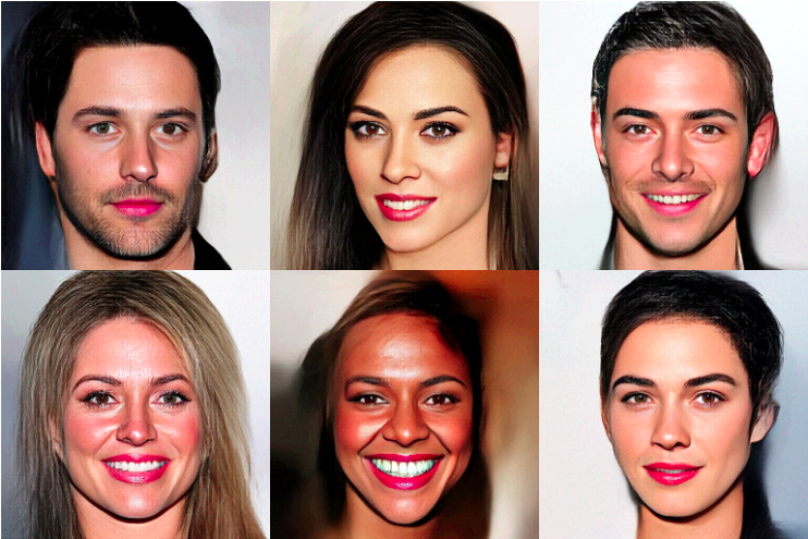
The glow model follows the same chain of formulas above, but combines a number of different layers designed for images, including invertible 1x1 convolutions, activation norm, and coupling layers (Dinh, Sohl-Dickstein, & Bengio, 2016). These layers are designed to increase the expressiveness of the flow model in the image domain. There are a number of other flow variants which approach learning these layers in diferent ways, such as neural spline flows (Durkan, Bekasov, Murray, & Papamakarios, 2019), radial flows and planar flows (Rezende & Mohamed, 2015). Flows have even found use in speeding up other trained models, such as Parallel Wavenet (Oord et al., 2018) which has found use in speech generation systems.

While normalizing flows involve a very exact and stable training procedure, they come with several downsides. First, all layers within a flow must be invertible and the log determinant must be easy to calculate for use of the change-of-variables formula. These conditions restrict flow layers and in practice, and can reduce their effectiveness. A second challenge of flows is that they cannot ignore infrequent modes of data in the training set. Later models like GANs can focus on more common data samples and increase their quality. If a flow assigns near zero probability to an infrequent example, the cross entropy loss value will be near infinity. This could potentially pose a challenge on multi-modal data distributions with outliers. (Kobyzev, Prince, & Brubaker, 2019) gives a more in-depth view of flows and their various forms.

Variational Autoencoders

The normalizing flow above attempts to maximize the probability of data $x$ produced from a latent vector $z$. This is an exact method of maximization. Variational Autoencoders (VAEs) do not attempt to maximize the probability of data $x$ directly, rather they try to maximize a lower-bound of it (Kingma & Welling, 2013). First, we imagine that from a datapoint $x$ we can deduce some latent variable $z$ with a known distribution (e.g. gaussian) which describes the data. This vector $z$ can be thought of as a summary of the data $x$, with a distribution we can sample from. So for images of faces it could encode pose, emotion, gender, etc.

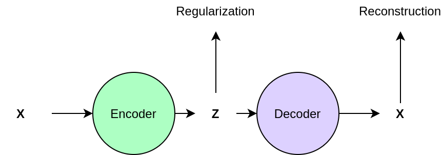
If only we knew the function $p(x\vert z)$, we could sample latent summary variables $z$ and “decode” them to a new data point $x$ - this would be our generative model. Even though our data points $x$ may be complex, we have related them to a simpler $z$-space where we can represent probability distributions more easily. This is very similar to the normalizing flows approach. Variational autoencoders achieve this using a learned probabilistic encoder to convert from $x$ to $z$-space, along with a learned deterministic decoder to convert from $z$-space back to $x$-space (reconstruction). Points within the $z$ space are regularized to be similar to a gaussian prior distribution to simplify the space and allow sampling. Thus, the diversity of the output generation is modeled in the $z$ domain, and the decoder deterministically maps each point $z$ to a point $x$ in the data domain. The pipeline looks as follows:

Assume that the conversion to these latent variables $z$ can be described by some unknown distribution $p(z\vert x)$ - we wish to model this “prior” distribution using our own “posterior” distribution $q(z\vert x)$ which we parameterize and learn from the data. As with normalizing flows, we seek to maximize the log probability of the data. The (log) probability of data $x$ can be expressed in terms of a lower bound $L$ for a positive-valued KL-divergence (dissimilarity) between the prior $p(z\vert x)$ and our posterior encoder $q(z\vert x)$.

$$\log q_\theta (x^{(i)}) = D_{KL}(q_\phi (z\vert x^{(i)}) \| p (z\vert x^{(i)})) + L(\theta, \phi, x^{(i)})$$

Notice that if our model $q(z\vert x)$ perfectly matches the selected prior distribution $p(z\vert x)$, then this lower-bound $L$ is equal to the true log probability we wish to maximize. We set our known prior $p(z\vert x) = p(x)$ to be independent of $x$ and solve:

$$\log q_\theta (x^{(i)}) \geq L(\theta, \phi, x^{(i)}) = E_{\log q_\phi (z\vert x)}[-\log q_\phi (z\vert x) + \log q_\theta (x, z)]$$

Solving for the lower bound:

$$L(\theta, \phi, x^{(i)}) = -D_{KL} (q_\phi (z\vert x^{(i)}) \| p (z)) + E_{q_\phi (z\vert x^{(i)})}[\log q_\theta (x^{(i)} \vert z)]$$

The variational autoencoder seeks to minimize this objective for encoder $q(z\vert x)$ and decoder $p(x\vert z)$. If the first term is minimized, then our encoder $q(z\vert x) = p(z)$. If the second term is minimized, our decoder $p(x\vert z)$ has found a conversion between $z$ and $x$. Thus the final result is a balance between the first term which simplifies $q(z\vert x)$ and the second term which requires it to hold useful information for reconstruction of $x$. After training, we then sample a vector $z$ from the prior $p(z)$ and pass it through our decoder to produce a sample! We have a generative model.

The reparameterization trick attempts to give a solid form to the prior $p(z)$ and posterior $q(z\vert x)$. The authors choose a multivariate gaussian with mean zero and standard deviation one along each dimension as the prior. This is simple enough that we can sample when we want to decode an output data point $x$.

$$z \sim p(z\vert x) = \mathcal{N}(\mu,\sigma^2)$$

Then, the posterior distribution $q(z\vert x)$ is parameterized by learned mean and standard deviation vectors $\mu$ and $\sigma$ produced by the encoder. The output of the encoder which represents $q(z\vert x)$ and is sampled as follows:

$$z = \mu + \sigma \epsilon$$

where epsilon is drawn from a multivariate normal distribution \mathcal{N}(0,1). The purpose of this parameterization is to express the output of the encoder as a manipulation of a gaussian distribution which can be shaped using $\mu$ and $\sigma$ produced by the encoder, giving the VAE the ability to represent $z$ as a latent distribution.

We add an epsilon noise vector $\epsilon$ used such that $q(z\vert x)$ is not deterministic. While other forms can be chosen, many VAE works follow a similar format of matching means and standard deviations between prior and posterior gaussian distributions (Serban et al., 2017). These are simple enough that we can calculate the KL-divergence term analytically. Combining the lower bound discussed above and this reparameterization trick, we can derive the exact function we maximize:

$$L(\theta,\phi;x^{(i)}) \simeq \dfrac{1}{2}\sum_{j=1}^{J}(1+\log ((\sigma_j^{(i)})^2)) - (\mu_j^{(i)})^2 - (\sigma_j^{(i)})^2)+\dfrac{1}{L}\sum_{l=1}^L \log q_\theta (x^{(i)}\vert z^{(i,l)})$$

for $z^{(i,l)}=\mu^{(i)}+\sigma^{(i)} \odot \epsilon^{(l)}$ and $\epsilon^{(l)} \sim \mathcal{N}(0,I)$. The first term is the KL-loss objective, which converges $q(z\vert x)$ to $p(z)$. Since the posterior distribution is just a transformed gaussian, this term can be solved by setting $\mu_j = 0$ and $\sigma_j = 1$. The second term is a reconstruction loss which maximizes $p(x\vert z)$, or the ability to recover the sample $x$ from latent $z$. It is important to remember here that our decoder is deterministic (in the image domain), and that the reconstruction term becomes a mean-squared error loss in this case. All variation in the output comes from the latent variable $z$. We sample from $p(z)$ and run this through the decoder $p(x\vert z)$ to produce a data point. Pretty neat!

The variational autoencoder seems to have some downsides. First, in this formulation it seems to be impossible to maximize both the KL-loss term and the reconstruction loss at the same time for this prior. If we satisfy the KL-divergence loss (first term), then encoder $q(z\vert x) = p(z)$ and our encoder has lost all information about $x$, effectively separating the relationship between $x$ and $z$ and forcing our decoder to maximize $p(x\vert z) = p(x)$. Since our decoder is a deterministic model, we do poorly and are back at the problem of representing $p(x)$ without a random variable $z$. It is thus desirable to have a balance between the KL-divergence objective and the reconstruction loss, but this reduces reconstruction performance and can cause blurring effects in images or grammar errors in output sentences. Overall, this balance can reduce the capacity of the VAE to generate high quality images in certain cases. However, VAEs place no constraint on the generator architecture, a straight-forward to train, and can even perform approximate probability density estimation. (Higgins et al., 2017) perform an extensive analysis on the weighting between KL-divergence and reconstruction objectives and the resulting images, feel free to take a look!

Variational autoencoders have been used extensively in a variety of domains. They have found use in modeling semantic sentence spaces, allowing for interpolation between sentences (Bowman et al., 2015), video generation (Lee et al., 2018), text planning (Yarats & Lewis, 2018), image generation (Razavi, van den Oord, & Vinyals, 2019) and more. Despite concerns of image blurring, (Razavi, van den Oord, & Vinyals, 2019) have recently been able to generate high-quality images that compete with the best Generative Adversarial Network architectures, which we discuss in the next section.

Generative Adversarial Networks

Previous models attempt to maximize either the probability of the data distribution (as in normalizing flows), or a lower bound of it (as in VAEs). Generative Adversarial Networks (Goodfellow et al., 2014) attempt to model the data distribution through a clever adversarial competitive game between two agents. We first form a model $G$ which will attempt to generate samples of our data (such as pictures of cats). Similar to models above, it takes as input a noise variable (vector) which it manipulates into an output image, etc. In the beginning of training it is randomly initialized and is very bad at this task. Next, we forge a model $D$ which will inform our generator $G$ on how to generate proper samples. The game works as follows: The generator generates a sample $x_g$. We then draw a true sample (e.g. a cat photo) from the dataset we wish to learn from. We present each of these separately to the discriminator $D$, and ask it to properly classify which is the fake image.

Fig. 4. Discriminator receives real and fake data (images) from the dataset and the generator.

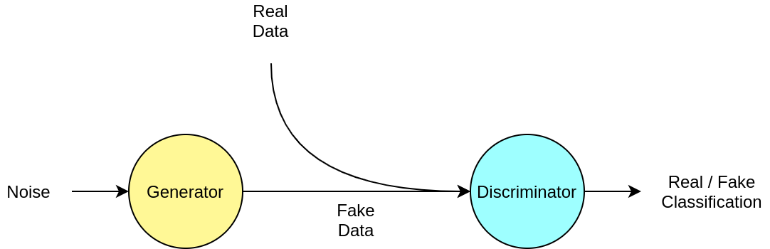
Over time, the discriminator then begins to get very good at discriminating between these samples. Simultaneously, we ask the generator to confuse the discriminator by making generated samples more realistic, or closer to the true distribution. This game continues, with the generator producing higher quality images while the discriminator becomes better at telling them apart from real ones. Theoretically, at convergence the generator will have captured the true distribution of the data $p(x)$ and we can generate new samples using G. This is intuitive; the only way for the discriminator to not be able to tell the difference between real and generated images is if they are identical (or close to it). This mini-max “game” can be formulated through the following objective:

$$(G,D)=\min_G \max_D V(D,G) = E_{x \sim p_{data}(x)}[log D(x)] + E_{z \sim p_z(z)}[log(1-D(G(z)))]$$

This formula shows that the generator and discriminator maximize and minimize the same objective, which is cross entropy loss over classification of data samples as real or fake by the discriminator. Other GAN papers attempt to reformulate this objective for better stability such as the Wasserstein GAN (Arjovsky, Chintala, & Bottou, 2017) and LSGAN (Mao et al., 2017). For a convergence analysis of different GANs, check out (Mescheder, Geiger, & Nowozin, 2018). Currently, generative adversarial networks are seeing the widest use as generative models in the image domain.

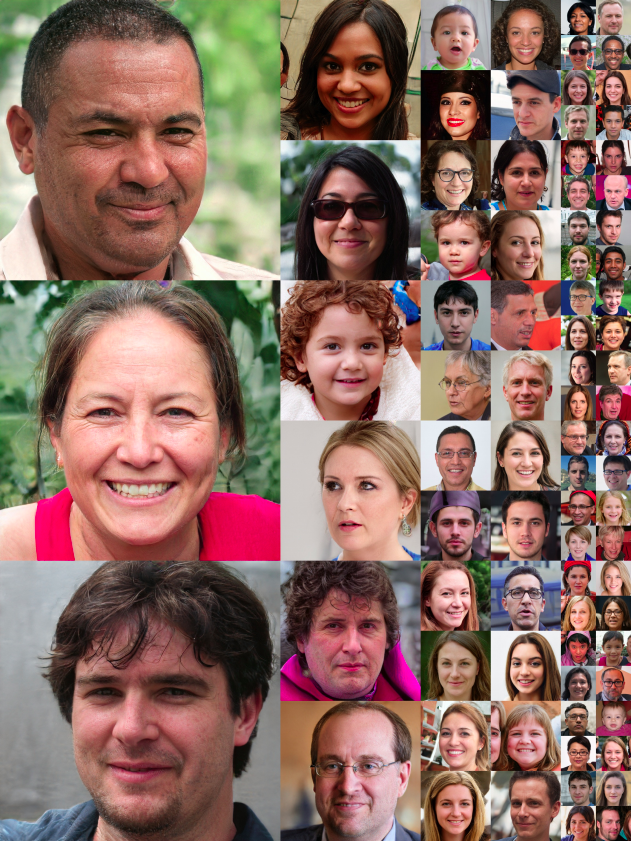
Through significant compute power, GANs have been trained to do some pretty cool things. NVidia has recently developed a style-based GAN (Karras, Laine, & Aila, 2019) capable of producing photo-realistic images. This model combines input style vectors at multiple hierarchies to change both high and low-level details of the output image. It is based on the progressively-growing GAN architecture (Karras, Aila, Laine, & Lehtinen, 2017) which generates an image at low-resolutions first for improved stability. Check these out:

Fig. 5. These humans have never existed, but rather have been generated from scratch by a large GAN. Scary?

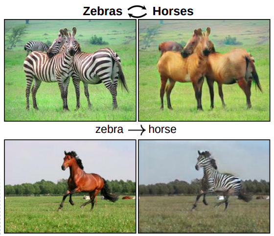
Another interesting model is CycleGAN (Zhu, Park, Isola, & Efros, 2017) which attempts to a learn a mapping between not one but two data distributions with no aligned data (no pairs, just stacks of two types of images). For example, they successfully learn a mapping from zebra photos to horse photos and between different seasons. However, this system is better at replacing textures than morphing object shapes, and so does not work as well with other objects such as apples and oranges.

Overall, generative adversarial networks are the most popular model because they produce high-quality images in one pass and do not place any constraints on the architecture of the generator. However, it is often observed that GANs can be unstable for smaller batch sizes when not properly tuned, and can be prone to mode collapse (Kodali, Abernethy, Hays, & Kira, n.d.).

Fig. 6. A model that converts between pictures of horses and zebras! Notice that for the most part, only textures change.

Overall, GANs are powerful because they do not place restrictions on the generator, they are conceptually simple, and they are fast during training and inference time. As for downsides, GANs do not tell you the estimated probability of samples you generate, unlike normalizing flows which give the exact density. Even more, they can be unstable to train for multi-modal data and smaller batches sizes. That being said, they are extremely popular in computer vision and have contributed impressive results to a variety of problem domains including style transfer (Xu, Wilber, Fang, Hertzmann, & Jin, 2018) and video generation (Clark, Donahue, & Simonyan, 2019).

Denoising Score Matching

Here we introduce a method of generation that is not as well known but still interesting as it takes a different perspective on generation. Denoising score matching (DSM) takes yet another approach to learning the data distribution $p(x)$. Instead of learning to represent the density of different samples, DSM attempts to learn the gradient of the probability distribution. Although this method has been used in the past to model distributions, recently (Song & Ermon, 2019) use DSM to generate natural images by learning the gradient of the distribution at multiple levels of noise. This gradient can be thought of as a compass in data/image space pointing in the direction of highest probability (toward the data manifold). This gradient can be learned using the denoising score matching objective:

$$L = \dfrac{1}{2}E_{q_\sigma (\tilde{x}\vert x)p_{data}(x)}[\vert s_\theta (\tilde{x}) - \nabla_{\tilde{x}}\log q_\sigma (\tilde{x}\vert x)\vert ^2_2]$$

This objective can be loosely interpreted as taking an input data point $x$ and adding a bit of noise to it as $\tilde{x}$ according to a noise distribution $q$, then asking the model to determine the direction the point came from and how far it traveled - this prediction will point toward the data distribution. It is proven that minimizing this equation satisfies

$$s_\theta (\tilde{x})=\nabla_{\tilde{x}} p_{data}(x)$$

and your score function has modeled the gradient. Once the gradient is learned, the authors use a procedure called Langevin dynamics to iteratively converge to a data sample using the following iterative procedure. This procedure begins from a randomly initialized point of low probability and follows the gradient before settling on a point of higher probability. Starting from randomly sampled datapoint $x_{t-1}$, we compute the next time step:

$$x_t = x_{t-1}+\dfrac{\epsilon}{2}\nabla_{x}\log p(x_{t-1}) + \sqrt{\epsilon} z_t$$

where $z_t$ is sampled from a multivariate gaussian distribution $\mathcal{N}(0,I)$. As $t\rightarrow \infty$, the distribution of $x_t$ approaches $p(x)$ and so we are producing new samples from the data!

Fig. 7. Process of Langevin dynamics recovering different faces from random noise.

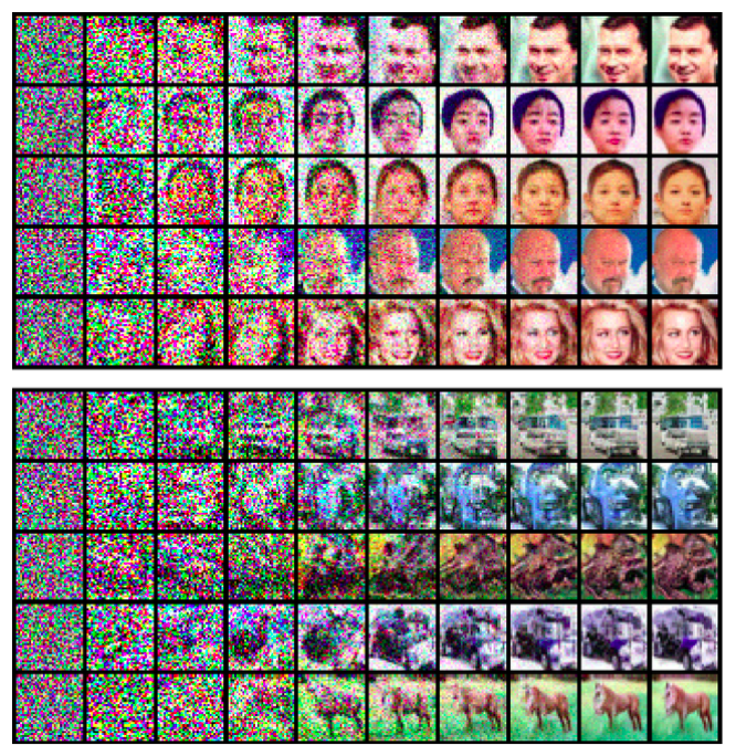
This sampling technique can be used to generate different samples, the authors of apply DSM to generate images of faces. This approach has the benefit that it does not require two separate models to learn the distribution (as in GANs and VAEs) and it does not place any constraints on the model architecture (as in normalizing flows). However, this model was only demonstrated to produce low-dimensional images, it is unclear if this scales to high-definition samples as GANs and normalizing flows have been proven to generate. In addition, this method is slow during inference because it requires running the model iteratively through the Langevin dynamics procedure. It would be interesting if this approach could be combined with another model to produce faster inference generation. Overall, this technique is interesting because score matching approaches the problem of learning probability distributions by learning the distribution implicitly instead of explicitly.

Conclusion

In this article we introduced a variety of architectures for generating data samples in different domains such as images and language. Each model has different properties, costs and benefits to consider for your application. Good luck!

References

1. Zhu, J.-Y., Park, T., Isola, P., & Efros, A. A. (2017). Unpaired image-to-image translation using cycle-consistent adversarial networks. Proceedings of the IEEE international conference on computer vision, 2223–2232.
2. Yarats, D., & Lewis, M. (2018). Hierarchical text generation and planning for strategic dialogue. International Conference on Machine Learning, 5591–5599.
3. Xu, Z., Wilber, M., Fang, C., Hertzmann, A., & Jin, H. (2018). Learning from multi-domain artistic images for arbitrary style transfer. ArXiv Preprint ArXiv:1805.09987.
4. Song, Y., & Ermon, S. (2019). Generative modeling by estimating gradients of the data distribution. Advances in Neural Information Processing Systems, 11895–11907.
5. Serban, I. V., Sordoni, A., Lowe, R., Charlin, L., Pineau, J., Courville, A., & Bengio, Y. (2017). A hierarchical latent variable encoder-decoder model for generating dialogues. Thirty-First AAAI Conference on Artificial Intelligence.
6. Rezende, D. J., & Mohamed, S. (2015). Variational inference with normalizing flows. ArXiv Preprint ArXiv:1505.05770.
7. Razavi, A., van den Oord, A., & Vinyals, O. (2019). Generating diverse high-fidelity images with vq-vae-2. Advances in Neural Information Processing Systems, 14866–14876.
8. Oord, A., Li, Y., Babuschkin, I., Simonyan, K., Vinyals, O., Kavukcuoglu, K., … others. (2018). Parallel wavenet: Fast high-fidelity speech synthesis. International conference on machine learning, 3918–3926.
9. Mescheder, L., Geiger, A., & Nowozin, S. (2018). Which training methods for GANs do actually converge? ArXiv Preprint ArXiv:1801.04406.
10. Mao, X., Li, Q., Xie, H., Lau, R. Y. K., Wang, Z., & Paul Smolley, S. (2017). Least squares generative adversarial networks. Proceedings of the IEEE International Conference on Computer Vision, 2794–2802.
11. Lee, A. X., Zhang, R., Ebert, F., Abbeel, P., Finn, C., & Levine, S. (2018). Stochastic adversarial video prediction. ArXiv Preprint ArXiv:1804.01523.
12. Kodali, N., Abernethy, J., Hays, J., & Kira, Z. On Convergence and Stability of GANs. arXiv 2017. ArXiv Preprint ArXiv:1705.07215.
13. Kobyzev, I., Prince, S., & Brubaker, M. A. (2019). Normalizing flows: Introduction and ideas. ArXiv Preprint ArXiv:1908.09257.
14. Kingma, D. P., & Dhariwal, P. (2018). Glow: Generative flow with invertible 1x1 convolutions. Advances in Neural Information Processing Systems, 10215–10224.
15. Kingma, D. P., & Welling, M. (2013). Auto-encoding variational bayes. ArXiv Preprint ArXiv:1312.6114.
16. Karras, T., Laine, S., & Aila, T. (2019). A style-based generator architecture for generative adversarial networks. Proceedings of the IEEE Conference on Computer Vision and Pattern Recognition, 4401–4410.
17. Karras, T., Aila, T., Laine, S., & Lehtinen, J. (2017). Progressive growing of gans for improved quality, stability, and variation. ArXiv Preprint ArXiv:1710.10196.
18. Higgins, I., Matthey, L., Pal, A., Burgess, C., Glorot, X., Botvinick, M., … Lerchner, A. (2017). beta-VAE: Learning Basic Visual Concepts with a Constrained Variational Framework. Iclr, 2(5), 6.
19. Goodfellow, I., Pouget-Abadie, J., Mirza, M., Xu, B., Warde-Farley, D., Ozair, S., … Bengio, Y. (2014). Generative adversarial nets. Advances in neural information processing systems, 2672–2680.
20. Durkan, C., Bekasov, A., Murray, I., & Papamakarios, G. (2019). Neural spline flows. Advances in Neural Information Processing Systems, 7509–7520.
21. Dinh, L., Sohl-Dickstein, J., & Bengio, S. (2016). Density estimation using real nvp. ArXiv Preprint ArXiv:1605.08803.
22. Clark, A., Donahue, J., & Simonyan, K. (2019). Adversarial video generation on complex datasets. ArXiv, arXiv–1907.
23. Bowman, S. R., Vilnis, L., Vinyals, O., Dai, A. M., Jozefowicz, R., & Bengio, S. (2015). Generating sentences from a continuous space. ArXiv Preprint ArXiv:1511.06349.
24. Arjovsky, M., Chintala, S., & Bottou, L. (2017). Wasserstein gan. ArXiv Preprint ArXiv:1701.07875.