Parameter Efficient Pre-Training: Comparing ReLoRA and GaLore
06 May 2024 • 8 mins

Parameter Efficient Pre-Training (PEPT)
As the size and complexity of large language models (LLMs) continue to grow, so does the demand for computational resources to train them. With billions of parameters, training these models becomes increasingly challenging due to the high cost and resource constraints. In response to these challenges, parameter-efficient fine-tuning (PEFT) methods have emerged to fine-tune billion-scale LLMs, for specific tasks, on a single GPU. This raises the question: can we use parameter-efficient training methods and achieve similar efficiency gains during the pre-training stage too?
Parameter-efficient pre-training (PEPT) is an emerging area of research that explores techniques for pre-training LLMs with fewer parameters. Multiple studies suggest that neural network training is either low-rank or has multiple phrases with initially high-rank and subsequent low-rank training (Aghajanyan et al., 2021, Arora et al., 2019, Frankle et al., 2019). This suggests that parameter-efficient training methods can be used to pre-train LLMs.
ReLoRA (Lialin et. al, 2023) is the first parameter-efficient training method used to pre-train large language models. ReLoRA uses LoRA decomposition, merges and resets the values of the LoRA matrices multiple times during training, increasing the total rank of the update. Another recent advance in PEPT is GaLore (Zhao et. al, 2024). In GaLore, the gradient is projected into its lower rank form, updated using an optimizer, and projected back to its original shape, reducing the memory requirement for pre-training LLMs.
This blog discusses ReLoRA and GaLore, explaining their core concepts, and key differences.
ReLoRA: High-Rank Training Through Low-Rank Updates
ReLoRA uses LoRA (Hu et al., 2022) decomposition technique where the pre-trained model weights are frozen and trainable rank decomposition matrices (WA, WB) are injected into each attention and MLP layer of the LLM. However in LoRA, the rank of the matrix is restricted by the rank r (given below), and the new trainable parameters (WA and WB) are merged back to the original matrices only after the end of the training.
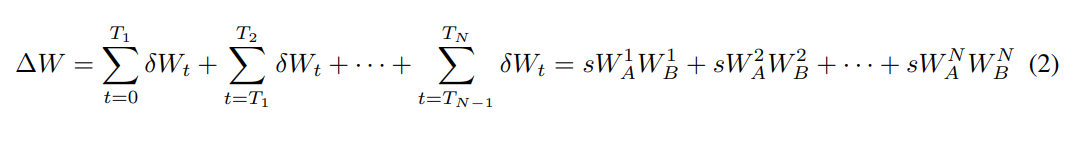
To increase the total rank of the updates, ReLoRA uses the property of the rank of the sum of two matrices: rank(A + B) ≤ rank(A) + rank(B). ReLoRA merges the LoRA matrices with the original matrices multiple times during training leading to the high rank update (ΔW).
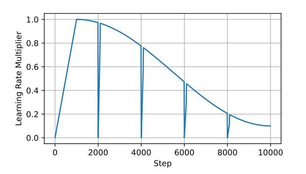
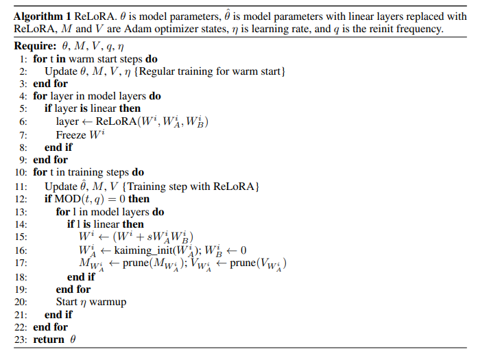
While ReLoRA's low-rank updates and merge-and-reinitialize approach offer efficiency gains and high-rank updates, there are a few challenges. Since the optimizer relies on ADAM, the updates are still highly correlated. ReLoRA performs a partial reset (>90%) of the optimizer state, focusing on pruning magnitudes. This helps break the correlation between updates and ensures the optimization process remains stable. However, this led to an exploding loss. A solution to this problem is to use a jagged learning rate scheduler, where on every optimizer reset, the learning rate is set to zero and a quick (50-100 steps) learning rate warm-up is performed to bring it back to the cosine schedule (Figure 1). This prevents the loss function from diverging significantly after the optimizer reset. Additionally, ReLoRA uses a warm start to gain better performance. During warm start, the model begins with a full-rank training phase for a portion of the training process (typically around 25%) before switching to the low-rank training phase.
ReLoRA is described in Algorithm 1.
GaLore: Memory-Efficient LLM Training by Gradient Low-Rank Projection
GaLore is a memory-efficient pre-training technique where gradients of the weight matrices are projected into low-rank form, updated using an optimizer, and projected back to the original gradient shape, which is then used to update the model weights. This technique is based on lemmas and theorems discussed in the paper. The main lemma and theorem are described below.
- Lemma: Gradient becomes low-rank during training
If the gradient is of form Gt = A - BWtC, with constant A and PSD matrices B and C, the gradient G converges to rank-1 exponentially, suggesting that the gradient of the given form becomes low rank during training. - Theorem: Gradient Form of reversible models
A reversible network with L2 objective has the gradient of form Gt = A - BWtC. The definition and proof of reversible networks are discussed in the paper. It is shown that the Feed Forward networks and softmax loss function are reversible networks, thus having a gradient of the given form. Attention may or may not be a reversible network.
As LLMs are made of feed-forward networks and activation functions, based on the above lemma and theorem and its proof, it is implied that LLMs have a gradient of form Gt = A - BWtC. It is assumed the attention is also a reversible network. As the gradient is of the given form, the gradient becomes low rank as training progresses.
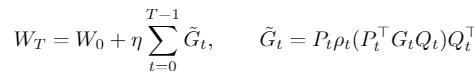
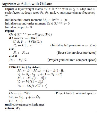
GaLore decomposes the gradient G⎯ into P, a low-rank gradient G, and Q matrices using SVD. P (shape m x r) and Q (shape r x n) are projection matrices and r denotes the rank. During each training step, either P or Q is utilized based on whether m is less than or equal to n. The low-rank gradient G⎯, is updated using an optimizer (e.g. AdamW). Subsequently, the updated G⎯ is projected back to the original space using the transpose of projection matrices P or Q.
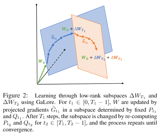
To facilitate efficient learning, GaLore employs a strategy of subspace switching by reinitializing the projection matrices after a predefined number of steps, known as the update frequency. This approach allows the model to learn within a specific subspace for a set duration before transitioning to another subspace with different initialization parameters for the projection matrices. GaLore uses the current step gradient to re-initialize the projection matrices. Figure 2 shows a geometric interpretation of the low-rank subspace updates in GaLore.
The algorithm is given here:
Comparison between ReLoRA and GaLore
The table below, summarizes the key differences between ReLoRA and GaLore, two parameter-efficient pre-training techniques discussed earlier.
| ReLoRA | GaLore | |
|---|---|---|
| Decomposition used | LoRA | SVD |
| Perplexity difference: Full rank v/s | 0.44 (1.3B model) | 0.08 (1B model) |
| Tokens trained on | 23.1B | 13.1B |
| Weight equation | Wt = Wt-1 + AB | Wt = Wt-1 + PTGP if m<=n |
| Gradient form | No conditions | Gt = A - BWtC, with constant A and PSD matrices B and C |
| Changes subspace using | Using Optimizer reset | Re-initialization of P |
| Number of matrices trained | 2, A (m x r) and B (r x n) | 1, G (m x r) or (r x n) Able to use higher rank as only one matrix is being trained |
| Additional hyperparameters | 3, optimizer state pruning percentage, reset frequency, rank | 3, rank, projection rate, update frequency |
| Memory required (1B scale) | 6.17 G | 4.38 G |
| Throughput | 7.4 ex/sec (given 1 RTX 3090, 25G) | 6.3 ex/sec (given 1 RTX 4090, 25G) |
| Warm-start required | Yes | No |
| Rank (1B scale) | 128 | 512 (at rank 1024, GaLore performs better than full training) |
| Compatible with | - | 8-bit optimizers, Per-layer weight updates |
| Optimizers | AdamW | 8-bit Adam, AdamW, Adafactor |
- Decomposition: ReLoRA uses LoRA decomposition to approximate low rank updates, while GaLore uses Singular Value Decomposition (SVD).
- Perplexity difference (Full rank vs. Low rank): This metric measures how well the model predicts the next word in a sequence. Lower perplexity indicates better performance. The table shows the difference in perplexity achieved by each method when trained with a full-rank model compared to a lower-rank method. ReLoRA shows a larger difference (0.44) for a 1.3B parameter model, while GaLore shows a smaller difference (0.08) for a 1B parameter model.
- Tokens trained on: This indicates the number of words used to train the model. The perplexity comparison is done when the 1B scale model was trained on the given number of tokens.
- Weight equation: This shows how the model weights are updated during training using respective decomposition techniques.
- Gradient form: ReLoRA has no specific conditions on the gradient form, while GaLore requires the gradient to be in a specific form (Gt = A - BWtC).
- Changes subspace using: ReLoRA changes the subspace by resetting the optimizer state, while GaLore does this by re-initializing a projection matrix (P).
- Number of matrices trained: ReLoRA trains two matrices (A and B), while GaLore trains one matrix (G). GaLore can potentially use a higher rank for this matrix since it only trains one.
- Additional hyperparameters: These are tuning knobs that control the training process. Both methods adds three additional hyperparameters.
- Memory required: This shows the amount of memory needed to train the model with each method (for a 1 billion parameter model). GaLore requires less memory than ReLoRA.
- Throughput: Throughput refers to the number of examples the model can process per second. This is measured on specific hardware (one RTX 3090 with 25G network bandwidth). ReLoRA shows higher throughput in this case.
- Warm-start required: Whether a full-rank training phase is needed before switching to low-rank training. ReLoRA requires a warmup, while GaLore does not.
- Rank: This is the target rank of the low-rank decomposition used by each method (for a 1 billion parameter model). GaLore can potentially use a higher rank and achieve better results (as shown at a rank of 1024).
- Compatible with: This indicates additional features supported by each method. GaLore works with certain optimizers and weight update methods that ReLoRA does not.
- Optimizers: These are the optimization algorithms used to train the models. GaLore offers a wider range of compatible optimizers.
ReLoRA and GaLore represent distinct approaches to parameter-efficient pre-training for LLMs. ReLoRA employs LoRA decomposition along with the warm-start phase, speeding up the training but having a higher memory utilization. Conversely, GaLore relies on Singular Value Decomposition (SVD), offering reduced memory requirements and the potential for higher ranks but reduced throughput. These methods diverge in their requirement of gradient forms, subspace changes, and the number of matrices trained, providing different options for LLM pre-training.
References
Lialin, V., Muckatira, S., Shivagunde, N., & Rumshisky, A. (2023). ReLoRA: High-Rank Training Through Low-Rank Updates.
Zhao, J., Zhang, Z., Chen, B., Wang, Z., Anandkumar, A., & Tian, Y. (2024). GaLore: Memory-Efficient LLM Training by Gradient Low-Rank Projection. ArXiv, abs/2403.03507.
Hu, E. J., Shen, Y., Wallis, P., Allen-Zhu, Z., Li, Y., Wang, S., Wang, L., & Chen, W. (2022). LoRA: Low-rank adaptation of large language models. In International Conference on Learning Representations. URL: https://openreview.net/forum?id=nZeVKeeFYf9.
Aghajanyan, A., Gupta, S., & Zettlemoyer, L. (2021). Intrinsic dimensionality explains the effectiveness of language model fine-tuning. In Proceedings of the 59th Annual Meeting of the Association for Computational Linguistics and the 11th International Joint Conference on Natural Language Processing (Volume 1: Long Papers), pages 7319–7328, Online, Aug. 2021. Association for Computational Linguistics. doi: 10.18653/v1/2021.acl-long. 568. URL: https://aclanthology.org/2021.acl-long.568.
Arora, S., Cohen, N., Hu, W., & Luo, Y. (2019). Implicit regularization in deep matrix factorization.
Frankle, J., Dziugaite, G. K., Roy, D. M., & Carbin, M. (2019). Stabilizing the lottery ticket hypothesis. arXiv e-prints, pages arXiv–1903.